Building Custom Batched Ensemble Weather Forecasting with NVIDIA Earth2Studio
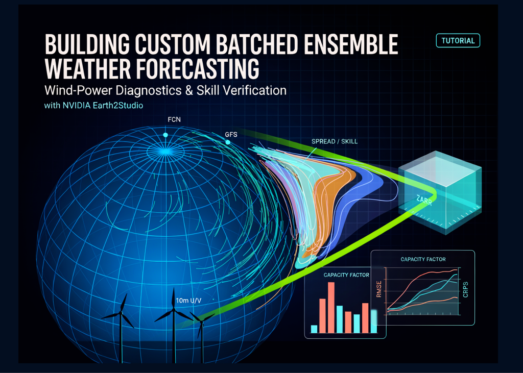
In this tutorial, we build an ensemble weather forecasting workflow with NVIDIA Earth2Studio. We install the required Earth2Studio components while preserving Colab’s existing CUDA-enabled PyTorch environment, load the FCN prognostic model, and retrieve atmospheric initial conditions from GFS. We then implement a custom wind-power diagnostic that converts 10-meter wind components into turbine capacity factors, along with a variable-scaled perturbation system that applies physically appropriate noise amplitudes to different atmospheric variables while retaining an unperturbed control member. Using Earth2Studio’s low-level iterator, coordinate-mapping, batching, and Zarr APIs, we construct our own ensemble execution pipeline, write forecast and diagnostic fields to a coordinate-aware data store, and verify the forecasts against GFS analyses using latitude-weighted RMSE, fair CRPS, ensemble spread, and spread-skill ratios. Finally, we visualize ensemble uncertainty through spatial maps, geopotential-height spaghetti contours, point-based fan charts, wind-capacity-factor forecasts, and lead-time skill curves.
if importlib.util.find_spec(“earth2studio”) is None:
import numpy as _np, torch as _torch
cfile = os.path.join(os.getcwd(), “e2s_constraints.txt”)
with open(cfile, “w”) as f:
f.write(f”torch=={_torch.__version__.split(‘+’)[0]}\n”)
f.write(f”numpy=={_np.__version__}\n”)
env = {**os.environ, “PIP_CONSTRAINT”: cfile}
subprocess.check_call(
[sys.executable, “-m”, “pip”, “install”, “-q”,
“earth2studio[fcn,data,perturbation,statistics]”], env=env)
print(“\n>>> Install done. If the imports below fail: Runtime > Restart session, re-run.\n”)
os.environ.setdefault(“EARTH2STUDIO_CACHE”, “/content/e2s_cache”)
os.makedirs(“outputs”, exist_ok=True)
from collections import OrderedDict
from datetime import datetime, timedelta, timezone
from tqdm.auto import tqdm
from earth2studio.data import GFS, fetch_data
from earth2studio.io import ZarrBackend
from earth2studio.models.batch import batch_coords, batch_func
from earth2studio.models.px import FCN
from earth2studio.statistics import rmse
from earth2studio.utils import handshake_coords, handshake_dim
from earth2studio.utils.coords import map_coords
from earth2studio.utils.time import to_time_array
from earth2studio.utils.type import CoordSystem
if DEVICE.type == “cpu”:
print(“!! No GPU detected — this will be very slow. Runtime > Change runtime type > T4 GPU”)
NENSEMBLE = 8
BATCH_SIZE = 2
NSTEPS = 8
SAVE_VARS = [“t2m”, “z500”, “u10m”, “v10m”, “tcwv”]
VERIFY_VARS = [“t2m”, “z500”, “u10m”]
INIT = (datetime.now(timezone.utc) – timedelta(days=7)).replace()
INIT_STR = INIT.strftime(“%Y-%m-%dT%H:%M:%S”)
POI = (“New Delhi”, 28.61, 77.21)
print(f”Initialization: {INIT_STR} | device: {DEVICE}”)
We install Earth2Studio while preserving Colab’s existing CUDA-enabled PyTorch and NumPy environment through package constraints. We configure the model cache, import the forecasting, data, statistics, plotting, and coordinate-management utilities, and detect the available compute device. We also define the ensemble size, batch size, forecast duration, saved variables, verification variables, initialization time, and New Delhi point of interest.
“””Turbine capacity factor [0,1] from 10 m winds via power-law shear + power curve.”””
def __init__(self, lat, lon, hub=100.0, alpha=0.143,
cut_in=3.0, rated=12.0, cut_out=25.0):
super().__init__()
self.lat, self.lon = lat, lon
self.hub, self.alpha = hub, alpha
self.cut_in, self.rated, self.cut_out = cut_in, rated, cut_out
def input_coords(self) -> CoordSystem:
return OrderedDict({
“batch”: np.empty(0),
“variable”: np.array([“u10m”, “v10m”]),
“lat”: self.lat,
“lon”: self.lon,
})
@batch_coords()
def output_coords(self, input_coords: CoordSystem) -> CoordSystem:
target = self.input_coords()
for i, (key, _) in enumerate(target.items()):
if key != “batch”:
handshake_dim(input_coords, key, i)
handshake_coords(input_coords, target, key)
oc = OrderedDict({
“batch”: np.empty(0),
“variable”: np.array([“wind_cf”]),
“lat”: self.lat,
“lon”: self.lon,
})
oc[“batch”] = input_coords[“batch”]
return oc
@batch_func()
def __call__(self, x: torch.Tensor, coords: CoordSystem):
oc = self.output_coords(coords)
u, v = x[…, 0:1, :, :], x[…, 1:2, :, :]
ws10 = torch.sqrt(u * u + v * v)
ws = ws10 * (self.hub / 10.0) ** self.alpha
ramp = (ws ** 3 – self.cut_in ** 3) / (self.rated ** 3 – self.cut_in ** 3)
cf = torch.zeros_like(ws)
cf = torch.where((ws >= self.cut_in) & (ws < self.rated), ramp.clamp(0, 1), cf)
cf = torch.where((ws >= self.rated) & (ws <= self.cut_out), torch.ones_like(cf), cf)
return cf, oc
class VariableScaledNoise:
“””Spatially correlated noise with per-variable amplitudes + control member.”””
def __init__(self, amplitudes: dict, default: float = 0.0, control_member: bool = True):
self.amplitudes, self.default, self.control = amplitudes, default, control_member
try:
from earth2studio.perturbation import SphericalGaussian
self.sampler, self.kind = SphericalGaussian(noise_amplitude=1.0), “SphericalGaussian”
except Exception:
from earth2studio.perturbation import Brown
self.sampler, self.kind = Brown(noise_amplitude=1.0), “Brown”
def __call__(self, x: torch.Tensor, coords: CoordSystem):
noise, _ = self.sampler(torch.zeros_like(x), coords)
vax = list(coords).index(“variable”)
amps = torch.tensor([self.amplitudes.get(str(v), self.default)
for v in coords[“variable”]], device=x.device, dtype=x.dtype)
shape = [1] * x.ndim; shape[vax] = amps.numel()
pert = noise * amps.reshape(shape)
if self.control and “ensemble” in coords:
eax = list(coords).index(“ensemble”)
mask = torch.tensor((np.asarray(coords[“ensemble”]) != 0).astype(np.float32),
device=x.device, dtype=x.dtype)
mshape = [1] * x.ndim; mshape[eax] = mask.numel()
pert = pert * mask.reshape(mshape)
return x + pert, coords
We create a custom diagnostic model that converts 10-meter wind components into hub-height wind speed and turbine capacity factor. We validate coordinate compatibility through Earth2Studio’s handshake utilities and support batched inputs with the provided decorators. We also implement variable-specific spatial perturbations that retain member zero as an unperturbed control forecast.
“””Write selected channels of a (…, variable, lat, lon) tensor to the IO backend.”””
vax = list(coords).index(“variable”)
sub = OrderedDict((k, v) for k, v in coords.items() if k != “variable”)
for name in names:
hit = np.where(np.asarray(coords[“variable”]) == name)[0]
if hit.size:
io.write(x.select(vax, int(hit[0])).cpu(), sub, name)
def run_ensemble(time, nsteps, nensemble, batch_size, prognostic, diagnostic,
perturbation, data, io, save_vars, device):
time = to_time_array(time)
ic = prognostic.input_coords()
x0, c0 = fetch_data(source=data, time=time, lead_time=ic[“lead_time”],
variable=ic[“variable”], device=device)
print(f”Initial condition tensor: {tuple(x0.shape)} dims={list(c0)}”)
oc = prognostic.output_coords(ic)
dt = oc[“lead_time”]
prog_vars = [v for v in save_vars if v in set(map(str, oc[“variable”]))]
total = OrderedDict({
“ensemble”: np.arange(nensemble),
“time”: time,
“lead_time”: np.asarray([dt * i for i in range(nsteps + 1)]).flatten(),
“lat”: oc[“lat”],
“lon”: oc[“lon”],
})
io.add_array(total, prog_vars + [“wind_cf”])
dx_target = OrderedDict((k, v) for k, v in diagnostic.input_coords().items() if k != “batch”)
nbatch = int(np.ceil(nensemble / batch_size))
with torch.inference_mode():
for b in tqdm(range(nbatch), desc=”ensemble batches”):
lo = b * batch_size
n = min(batch_size, nensemble – lo)
x = x0.unsqueeze(0).repeat(n, *([1] * x0.ndim))
coords = OrderedDict({“ensemble”: np.arange(lo, lo + n), **c0})
x, coords = perturbation(x, coords)
x, coords = map_coords(x, coords, ic)
for step, (xs, cs) in enumerate(prognostic.create_iterator(x, coords)):
write_vars(io, xs, cs, prog_vars)
xw, cw = map_coords(xs, cs, dx_target)
xw, cw = diagnostic(xw, cw)
write_vars(io, xw, cw, [“wind_cf”])
if step >= nsteps:
break
torch.cuda.empty_cache() if device.type == “cuda” else None
return io
model = FCN.load_model(FCN.load_default_package()).to(DEVICE)
grid = model.output_coords(model.input_coords())
LAT, LON = grid[“lat”], grid[“lon”]
diagnostic = WindPowerCF(LAT, LON).to(DEVICE)
pert = VariableScaledNoise(
amplitudes={“t2m”: 0.20, “t850”: 0.20, “z500”: 40.0, “z850”: 25.0,
“u10m”: 0.25, “v10m”: 0.25, “u500”: 0.40, “v500”: 0.40, “tcwv”: 0.30},
default=0.0, control_member=True)
print(f”Perturbation sampler: {pert.kind}”)
io = ZarrBackend(file_name=”outputs/e2s_ensemble.zarr”,
chunks={“ensemble”: 1, “time”: 1, “lead_time”: 1},
backend_kwargs={“overwrite”: True})
io = run_ensemble([INIT_STR], NSTEPS, NENSEMBLE, BATCH_SIZE,
model, diagnostic, pert, GFS(), io, SAVE_VARS, DEVICE)
print(io.root.tree())
We define helper functions that select atmospheric channels and write them into a coordinate-aware Zarr backend. We build a custom batched ensemble loop that fetches GFS initial conditions, perturbs ensemble members, aligns coordinates, iterates the FCN model, and chains the wind-power diagnostic. We then load the model, initialize the diagnostic and perturbation components, execute the forecast, and inspect the resulting Zarr structure.

lead_h = leads.astype(“timedelta64[h]”).astype(int)
valid = to_time_array([INIT_STR])[0] + leads
truth, tc = fetch_data(source=GFS(), time=valid,
lead_time=np.array([np.timedelta64(0, “h”)]),
variable=np.array(VERIFY_VARS), device=”cpu”)
truth = truth[:, 0]
w = torch.cos(torch.deg2rad(torch.as_tensor(np.asarray(LAT), dtype=torch.float32)))
w2d = w[:, None].expand(len(LAT), len(LON)).contiguous()
mcoords = OrderedDict({“lead_time”: leads, “lat”: np.asarray(LAT), “lon”: np.asarray(LON)})
def fair_crps(ens, obs, weights):
“””Fair (unbiased) CRPS, lat-weighted. ens: (M, lat, lon), obs: (lat, lon).”””
M = ens.shape[0]
wn = weights / weights.sum()
skill = ((ens – obs).abs() * wn).sum(dim=(-2, -1)).mean()
spread = torch.zeros((), dtype=ens.dtype)
for i in range(M):
spread = spread + ((ens[i] – ens).abs() * wn).sum(dim=(-2, -1)).sum()
return (skill – spread / (2 * M * (M – 1))).item()
scores = {}
for k, var in enumerate(VERIFY_VARS):
fc = torch.as_tensor(np.asarray(io[var][:]))[:, 0].float()
ob = truth[:, k].float()
mean = fc.mean(0)
try:
metric = rmse(reduction_dimensions=[“lat”, “lon”], weights=w2d)
r, _ = metric(mean, mcoords, ob, mcoords)
r = r.numpy()
except Exception as e:
print(f”(built-in rmse unavailable: {e})”)
wn = (w2d / w2d.sum())
r = torch.sqrt((((mean – ob) ** 2) * wn).sum(dim=(-2, -1))).numpy()
wn = w2d / w2d.sum()
spread = torch.sqrt((fc.var(0, unbiased=True) * wn).sum(dim=(-2, -1))).numpy()
crps = np.array([fair_crps(fc[:, t], ob[t], w2d) for t in range(fc.shape[1])])
scores[var] = dict(rmse=r, spread=spread, crps=crps, fc=fc, obs=ob, mean=mean)
print(f”\n=== {var} ===”)
print(f”{‘lead[h]’:>8}{‘RMSE’:>12}{‘spread’:>12}{‘ratio’:>9}{‘CRPS’:>12}”)
for t in range(len(lead_h)):
ratio = spread[t] / r[t] if r[t] > 0 else np.nan
print(f”{lead_h[t]:>8}{r[t]:>12.3f}{spread[t]:>12.3f}{ratio:>9.2f}{crps[t]:>12.3f}”)
We retrieve GFS analyses for every forecast-valid time and use them as the reference data for verification. We calculate latitude-weighted RMSE, ensemble spread, fair CRPS, and spread-to-error ratios for temperature, geopotential height, and wind variables. We store the forecast fields and evaluation metrics in a structured dictionary and print lead-time skill summaries for each variable.
ilat = int(np.argmin(np.abs(lat_np – POI[1])))
ilon = int(np.argmin(np.abs(lon_np – (POI[2] % 360))))
last = -1
d = scores[“t2m”]
fields = [(d[“mean”][last].numpy() – 273.15, “ensemble mean t2m [C]”, “RdBu_r”, None),
(d[“fc”][:, last].std(0).numpy(), “ensemble spread [K]”, “magma”, None),
(d[“obs”][last].numpy() – 273.15, “GFS analysis [C]”, “RdBu_r”, None),
((d[“mean”][last] – d[“obs”][last]).numpy(), “mean error [K]”, “coolwarm”, 5)]
fig, axs = plt.subplots(2, 2, figsize=(15, 7), constrained_layout=True)
for ax, (f, title, cmap, lim) in zip(axs.ravel(), fields):
kw = dict(vmin=-lim, vmax=lim) if lim else {}
im = ax.pcolormesh(lon_np, lat_np, f, cmap=cmap, shading=”auto”, **kw)
ax.set_title(f”{title} — +{lead_h[last]} h”); plt.colorbar(im, ax=ax, shrink=0.85)
plt.show()
z = scores[“z500”][“fc”][:, last].numpy() / 9.81
la = (lat_np > 25) & (lat_np < 75)
lo = (lon_np > 280) | (lon_np < 40)
lon_shift = np.where(lon_np > 180, lon_np – 360, lon_np)
order = np.argsort(lon_shift[lo])
plt.figure(figsize=(11, 5))
for m in range(z.shape[0]):
sub = z[m][np.ix_(la, lo)][:, order]
plt.contour(lon_shift[lo][order], lat_np[la], sub, levels=[5520],
colors=[“k” if m == 0 else “C0”], linewidths=[2.0 if m == 0 else 0.8])
zo = scores[“z500”][“obs”][last].numpy() / 9.81
plt.contour(lon_shift[lo][order], lat_np[la], zo[np.ix_(la, lo)][:, order],
levels=[5520], colors=”crimson”, linewidths=2.5)
plt.title(f”z500 5520 m spaghetti at +{lead_h[last]} h ”
f”(black=control, blue=members, red=GFS analysis)”)
plt.xlabel(“lon”); plt.ylabel(“lat”); plt.show()
t2m_pt = scores[“t2m”][“fc”][:, :, ilat, ilon].numpy() – 273.15
obs_pt = scores[“t2m”][“obs”][:, ilat, ilon].numpy() – 273.15
cf_pt = np.asarray(io[“wind_cf”][:])[:, 0, :, ilat, ilon]
fig, (a1, a2) = plt.subplots(1, 2, figsize=(14, 4))
a1.fill_between(lead_h, t2m_pt.min(0), t2m_pt.max(0), alpha=0.25, label=”member range”)
a1.plot(lead_h, t2m_pt.mean(0), “o-“, label=”ensemble mean”)
a1.plot(lead_h, t2m_pt[0], “k–“, label=”control”)
a1.plot(lead_h, obs_pt, “r^-“, label=”GFS analysis”)
a1.set_title(f”2 m temperature — {POI[0]}”); a1.set_xlabel(“lead [h]”); a1.set_ylabel(“C”)
a1.legend(); a1.grid(alpha=.3)
a2.fill_between(lead_h, cf_pt.min(0), cf_pt.max(0), alpha=0.25, color=”seagreen”)
a2.plot(lead_h, cf_pt.mean(0), “o-“, color=”seagreen”)
a2.set_title(f”wind capacity factor (custom diagnostic) — {POI[0]}”)
a2.set_xlabel(“lead [h]”); a2.set_ylim(0, 1); a2.grid(alpha=.3)
plt.tight_layout(); plt.show()
fig, axs = plt.subplots(1, len(VERIFY_VARS), figsize=(5 * len(VERIFY_VARS), 3.6))
for ax, var in zip(np.atleast_1d(axs), VERIFY_VARS):
s = scores[var]
ax.plot(lead_h, s[“rmse”], “o-“, label=”RMSE (ens. mean)”)
ax.plot(lead_h, s[“spread”], “s–“, label=”spread”)
ax.plot(lead_h, s[“crps”], “^:”, label=”fair CRPS”)
ax.set_title(var); ax.set_xlabel(“lead [h]”); ax.grid(alpha=.3); ax.legend(fontsize=8)
plt.tight_layout(); plt.show()
import xarray as xr
ds = xr.open_zarr(“outputs/e2s_ensemble.zarr”)
print(ds)
We visualize ensemble behavior through temperature mean, spread, analysis, and error maps at the final forecast lead time. We generate geopotential-height spaghetti contours, a New Delhi temperature fan chart, a wind-capacity-factor forecast, and lead-time skill curves. We finally open the Zarr output with Xarray so that we can inspect, analyze, or export the complete ensemble dataset.
In conclusion, we established a flexible and extensible Earth2Studio workflow that goes beyond running a predefined ensemble function. We directly controlled initial-condition perturbation, member batching, model iteration, diagnostic chaining, coordinate alignment, data persistence, verification, and visualization within a single Colab environment. We also demonstrated how physically scaled perturbations and an unperturbed control member help us interpret ensemble spread. At the same time, RMSE, fair CRPS, and spread-skill diagnostics allow us to evaluate forecast accuracy and calibration across lead times. The resulting Zarr dataset preserves the complete ensemble structure and remains accessible through Xarray for further analysis or conversion. Because the workflow follows Earth2Studio’s component interfaces, we can extend it by replacing the prognostic model, changing the atmospheric data source, adding new diagnostics, increasing the ensemble size, or adopting asynchronous storage without redesigning the full forecasting pipeline.
Check out the FULL CODES here. Also, feel free to follow us on Twitter and don’t forget to join our 150k+ML SubReddit and Subscribe to our Newsletter. Wait! are you on telegram? now you can join us on telegram as well.
Need to partner with us for promoting your GitHub Repo OR Hugging Face Page OR Product Release OR Webinar etc.? Connect with us
Sana Hassan, a consulting intern at Marktechpost and dual-degree student at IIT Madras, is passionate about applying technology and AI to address real-world challenges. With a keen interest in solving practical problems, he brings a fresh perspective to the intersection of AI and real-life solutions.